100 Days Of ML Code — Day 099

Recap from day 098

In the past two days, we’ve talked briefly about how to calculate the storage space of digital audio data based on decisions we’ve made about bit width, the number of channels, and sampling rate. We’ve talked about ways to reduce that storage space through lossless file formats and lossy file formats and the implications of each.

You can catch up using the link below. 100 Days Of ML Code — Day 098 Recap from day 097medium.com

Today, we’re going to move onto something a little bit different but actually goes back to some of what we were talking about when we looked at timbre which is essentially how we create these frequency representations of sound that we’re looking at when we’re talking about timbre, the sonogram and the spectral view.

Frequency Domain Analysis

I want to cover a somewhat complex topic, but I think it’s really important for us to understand it which is how we get from the waveform representation of digital audio and where we have time on our x-axis and amplitude on our y-axis to the sonogram representation where we can see much more information about the frequency and the timbre content of the sound.

We’re going to talk about how we get away from the sonogram and the role the Fourier Theorem plays in that. We’re going to talk about how we kind of work around the limitations of the Fourier Theorem through a process of windowing Periodicization and fast forwarding transform in order to take any sound that we might want to look at and represent it as a sum of a series of sound waves.

We’ll talk about some implications of this algorithm in terms of particularly two parameters of the frame size and bin width but we need to think about very carefully as we’re configuring it because they have some serious implications in terms of what we get are zeroes.

From Waveform to Sonogram

It’s pretty obvious now that we know how sound is represented digitally on a computer. It’s pretty obvious how a waveform representation like the one seen in the image below comes about. You know, we simply take the successive amplitude values, and we kind of plot them over time on the x-axis and then we have our waveform, we can connect the dots if we want to make it look a little nicer.

Source

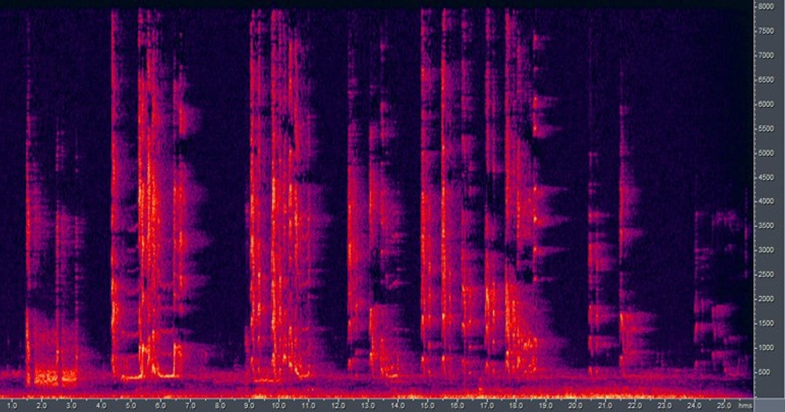
But how we get from the kind of representation above to the one seen below is not obvious because when we represent sound digitally we’re encoding a series of amplitude values over time we’re not including any information about the frequency at all. So that’s why we need to think about this a little bit more carefully and think about how we get to the representation seen below.

Source

So we’re going to revisit the Fourier Theorem which we looked at in the timbre article. I want to look at it in a little bit more depth now.

Just to recap we said the Fourier Theorem said that “any periodic waveform can be represented as a sum of sine waves at frequencies that are integer multiples of a fundamental frequency” and we looked at examples of this with a sawtooth wave and we looked at examples of the trombone sound of how we could kind of combine sine waves together.

I mean we wouldn’t hear them anymore as individual sine waves, but we’d hear them kind of coming together come possibly to create this single sound for us because of this special relationship they had to each other in terms of being integer multiples in a base frequency and because of the way that they were linked.

I also mentioned a really important limitation here. The periodic limitation. It only works for periodic waveforms like a perfect sine wave or a perfect square wave or something like that and that isn’t how sounds work in the real world. They’re not perfectly periodic. They don’t repeat a cycle infinitely over and over and over again without any variation.

So, that one problem is that we’ve gotten this spectra aspect of timbre but not the envelope of timbre, not the changing in time, aspect of it. The other problem is that when we say that the sum of sine waves, there’s an important caveat. It’s a potentially infinite number of sine waves may be required to do the summation and computers don’t tend to like infinity very much. They’re not continuous beings. They’re discrete; they do things as sets of zeros and ones.

So if we need potentially infinite number of sine waves to do the summation of sine waves, that’s also going to be really problematic for us and so what we do instead is, we use this basic idea of the Fourier Theorem but we tweak it a little bit, we kind of fake it out if you will pretend that we’re working periodic waves and we do process, it doesn’t do things perfectly but doesn’t use an infinite number of sine waves either to make the summation happen and so there are three stages to the process that I’m going to talk about in detail.

The Process

Windowing is when we take a waveform and split it up into tiny little bits. Then, we take each of those tiny little bits and we do this thing called Periodicization. There’s really nothing to this we just pretend that little bit repeats infinitely so that it’s a periodic sample and then on each of those little windows we apply a method called the Fast Fourier Transform which you’ll often see abbreviated as FFT and so we apply this process in order to convert our time domain set of amplitudes values into information about frequency.

So, I’m going to go through each of those steps in more detail tomorrow. That’s all for day 099. I hope you found this informative. Thank you for taking time out of your schedule and allowing me to be your guide on this journey. And until next time, be legendary.