


100 Days Of ML Code — Day 100
Recap from day 099
In day 099 we looked at something a little bit different but actually goes back to some of what we were talking about when we looked at timbre which is essentially how we create these frequency representations of sound that we’re looking at when we’re talking about timbre, the sonogram and the spectral view.
You can catch up using the link below. 100 Days Of ML Code — Day 099 Recap from day 098medium.com
Today, we’ll continue from where we left off In day 099
The Process
Windowing is when we take a waveform and split it up into tiny little bits. Then, we take each of those tiny little bits and we do this thing called Periodicization. There’s really nothing to this we just pretend that little bit repeats infinitely so that it’s a periodic sample and then on each of those little windows we apply a method called the Fast Fourier Transform which you’ll often see abbreviated as FFT and so we apply this process in order to convert our time domain set of amplitudes values into information about frequency. So, I’m going to go through each of those steps in more detail.
Windowing
The first step is Windowing so what we’re we do is divide the audio into equal size, overlapping frames. So, let me show you what I mean. We pick a number of samples that would be included in each frame. So, our frame size might be 1024 samples, for instance. So these are tiny frames. So 1024 samples if our sampling rate were 44,100 hertz is about 140th of a second. So tiny fractions of a second.
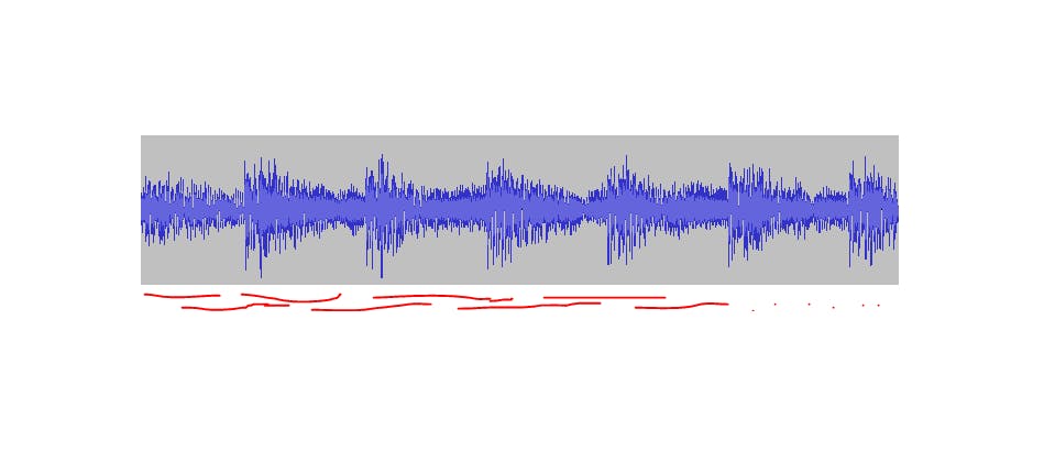
And so if we were taking the waveform seen above and splitting it up we might have the first red line that I’ve drawn under the waveform to be one and then we’re going to overlap them with each other. So the second red line under the first one might be another, the third line which is the line above the second line might be another and so on and so forth all the way through our file.
But it’s more complicated than what I’ve shown above actually because those are overlapping and we want smooth transitions from one to the next as we’re doing it, each of them kind of fades in and fades out.
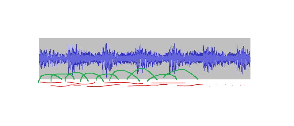
So the first one I’m going to fade in fade out with an amplitude envelope as represented by the green annotation as seen above. The next one we’ll fade in and fade out too, and so on. So there’s always one that’s kind of fading in and always one that’s kind of fading out with an overlap like the one seen above, and so on and so forth.
So that’s what windowing is, we end up with these windows that kind of fade in and fade out that are each a tiny fraction of a second long then we take each of those windows and, this is the easy part, we pretend that it’s a periodic function.
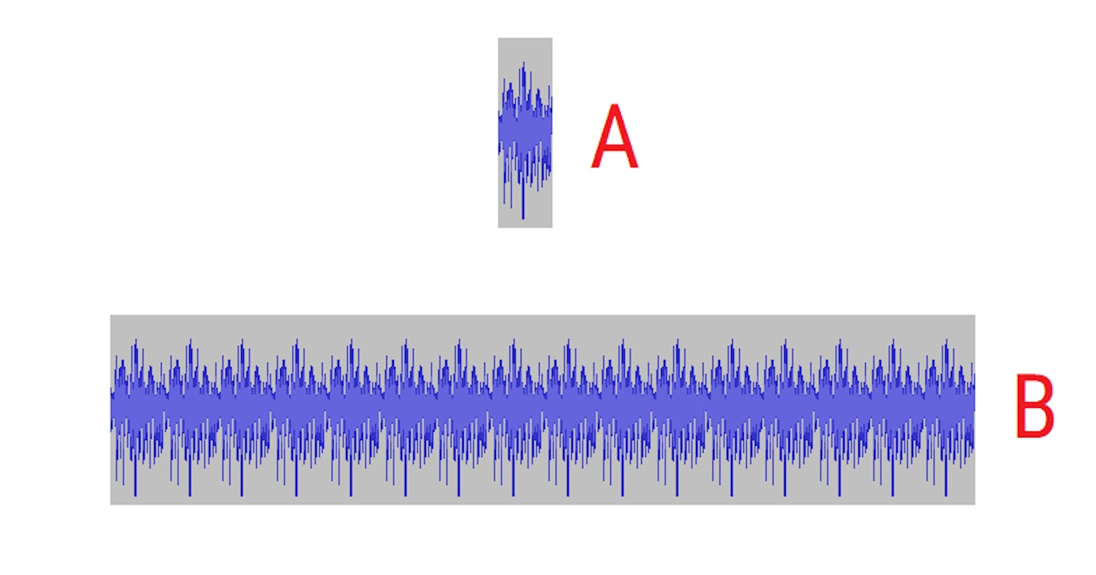
Periodicization
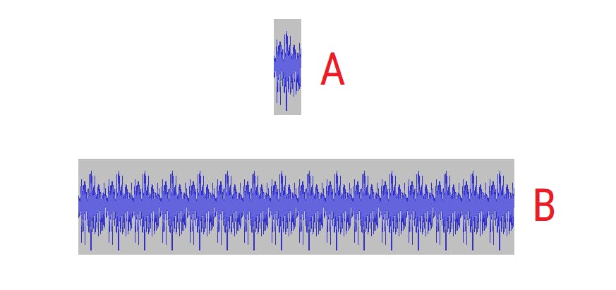
So we take a tiny little window like image A above, and we repeat it and we repeat it and we repeat it and we repeat and we repeat it and again, and again like in image B above. We just pretend that the repetition goes on forever. So now we’ve met the periodic requirement of the Fourier Theorem.
The Fast Fourier Transform
The final step is called The Fast Fourier Transform. The details of how this algorithm works are a little bit beyond the scope of this article. I encourage you to look up some more details if you’re interested, I’ll point you towards some references, but right now I just want to explain about, kind of pretend that it’s a black box. And explain kind of what goes in and what goes out.
What comes in are these amplitude samples overtime in the frame. So if our frame size is 1,024, we’d have 1,024 amplitude values that would go in. And what would come out are a set of amplitudes and phases for each frequency bin.
So in other words, I’m going to divide up my frequency space into a series of linearly spaced bins and then I’m going to look at what’s going on in each of those. How much energy is there in each of those bins? And also the phase of the sine wave it’s represented by each of those bins.
There are some simple ways to calculate how the algorithm does this and my number of frequency bins is half of my frame size and then the width between each of these bins from one to the next to the next is my Nyquist frequency, the highest frequency I can represent in my sampling rate, divided by my number of bins.
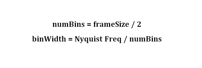
Let’s work through an example here just to make sure this is totally clear. So my frame size is 1,024 samples and my sampling rate is 44,100 Hertz then my Nyquist frequency would be 44,100 divided by 2 so 22,050. So then my number of bins is the frame size, 1024 divided by two. So that’s 512, and my bin width is going to be my Nyquist frequency that’s 22,050 Hertz divided by my number of bins, 512 This comes out to about 43 Hertz. It’s a little bit more than 43 Hertz. So that means that my frequency bins are going to be spaced zero, 43, 86, 129, so on and so forth all the way up to 22,050 Hertz.
So that’s how this stuff is divided up and then I have information at that point about what’s going on in each of those frequency areas and so you can see how it could generate a sonogram from there. I could take each of these frames and generate one vertical strip of frequency view in my sonogram based on that data that’s coming back
Issues and Tradeoffs
I want to talk about some of the issues with the process described above because it is not a perfect process.
First of all, it’s a Lossy process, I lose data in this process. If I do this fast Fourier Transform and then I go back to my waveform I’ve lost something in the process because I’ve split these things up into these linear frequency bins so I only know what’s happening with a very low resolution as they’re moving up in frequency and I also only know things about a fairly low resolution in terms of time because I only know what’s happening frame by frame by frame so 1,024 samples in the example we’ve been using at a time and so there’s actually a big trade-off when I pick my frame size.
In terms of how much resolution do I want in a time-domain versus how much do I want in the frequency domain if I want to know exactly when things are happening in time along my x-axis, I can pick a very low frame size so my frames are really tiny so I get a lot of time resolution or horizontally but then my bin width gets huge and so I know very little about what’s happening vertically in my frequency dimension.
If I want to know a lot vertically in my frequency dimension, I can pick a really high frame size but then there’s a lot of time that passes from one frame to the next to the next and so I lose a lot of resolution in the horizontal in the time domain.
The one point I wanted to make is that the frequency space is divided linearly but if you remember from psychoacoustics, we actually hear a pitch not linearly but logarithmically and so a lot of linear frequency bins are kind of wasted if you will on things very high up in frequency space. So half of the bins are for what we would hear as just the final octave of our frequency space so this isn’t a great match either, but that’s how this particular algorithm works.
Wow, you’re still here. It’s the 100th day. You deserve some accolades for hanging in here till the end. I hope you found the journey from day 001 to day 100 informative. Thank you for taking time out of your schedule and allowing me to be your guide on this journey. And until next time, be legendary.