100 Days Of ML Code — Day 090

Recap From Day 089

Day 089, we looked at Copying Analog And Digital.

You can catch up using the link below. 100 Days Of ML Code — Day 089 Recap From Day 088medium.com

If you lose your digital data if it gets corrupted, usually you’re just finished you have no semblance of the original left to work with at all, and so this is another point I wanted to make in this relationship between analog and digital.

So, to review here in the past two days we talked about the basic differences between analog and digital sound as continuous versus discreet representations of audio and we talked about those discreet samples of audio that we get in a digital representation of sound and the issue of horizontal resolution. Sampling rate, how many samples are we taking per second. Bit width, the vertical representation of how much resolution we are using to represent each amplitude dial, and how many channels of sound do we need. We talked about some implications of analog versus digital sound in copying audio and also in the kind of degradation and preservation of audio.

So, starting today and in the next couple of days, we’re going to delve into the three ideas of sampling rates, bit widths and channels in much more depth and look at some of the details about how we decide what we need in each of those domains.

Like I mentioned in the last paragraph, today, we’re going to delve into the question of sampling rate in much more detail and ask a simple question of how do we determine what the appropriate sampling rate is? We’ll, explain it a little bit more formally what a sampling rate is and we’ll look at the Nyquist Theorem, which gives us some guidance on picking a sampling rate.

Later on, we’ll also talk about foldover which is something that can happen usually that we usually don’t want to happen if you pick a bad sample that is too low for a particular project.

Sampling Rate

Sampling rate is very simply put, it’s the number of samples per second of digital audio.

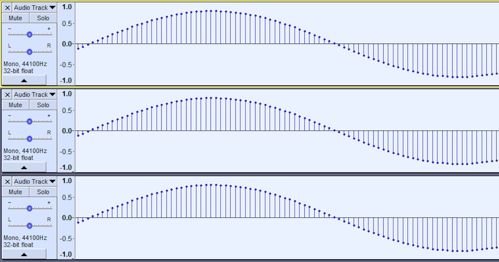
If you recall we have this kind of very zoomed-in sine wave as seen in the image above. Each of those dots is a sample. It’s simply asking, well, how many of those dots are we capturing every second. And because it is in terms of samples per second kind of metric, we actually use hertz to represent it, the same thing we had used to represent frequency.

For instance, if 8,000 hertz is our sampling rate, it simply means that we’re capturing 8,000 of these samples every second. So that’s how we talk about sampling rate. And now, how do we decide what our sampling rate should be? it’s actually fairly simple. We use something called the Nyquist Theorem, which is also sometimes known as the sampling theorem.

That’s all for day 090. I hope you found this informative. Thank you for taking time out of your schedule and allowing me to be your guide on this journey. And until next time, be legendary.