


Recap From Day 034
In day 034, we looked at working with audio input: Common audio features. We learned that Spectral Centroid tells us something about the timbre of a sound. Specifically, it gives us information about how bright a sound is. Visually, we can understand Spectral Centroid by imagining we have a frequency spectrum made out of solid object. The Centroid lies just under the center of mass of this object.
Today, we’ll continue from where we left off in day 034.
Working With Audio Input: Common Audio Features Continued
Constant Q Transform
“The constant-Q transform transforms a data series to the frequency domain. It is related to the Fourier transform and very closely related to the complex Morlet wavelet transform.” “The transform can be thought of as a series of logarithmically spaced filters fk, with the k-th filter having a spectral width δfk equal to a multiple of the previous filter’s width”
If you want information about pitch or timbre, but the peak frequency and Spectral Centroid don’t give you enough information, there is a nice middle ground in between those very simple features and using the full set of FFT magnitude values.
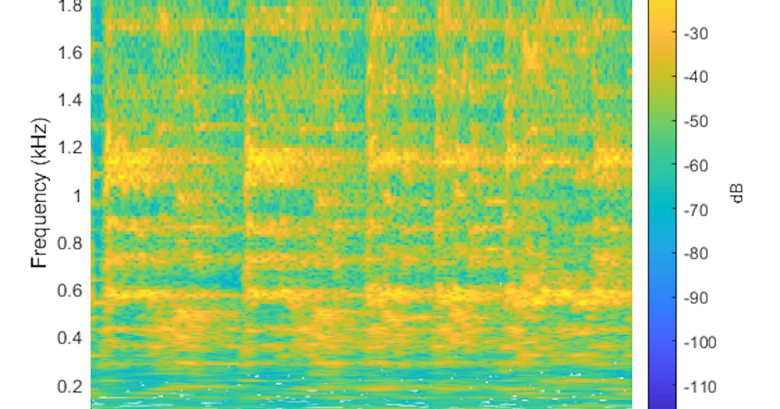
](https://cdn-images-1.medium.com/max/2000/1*ZrE_VsL0Y3XeIuyLVI3AiA.png)
The Constant Q transform gives us a nice, general-purpose feature vector in the middle ground between peak frequency and Spectral Centroid. Like the FFT, Constant Q gives us information about the strengths of the different frequencies present in our analysis window. However, Constant Q gives us logarithms spacing between these frequencies which sounds complicated until you realize that our human perception of frequency is basically logarithmic.
We can set up Constant Q to give us one frequency bin per octave, for example. And this can give us a low-dimensional feature vector that tells us something useful about the relative lowness or highness of the sound. Or, we could use Constant Q to give us twelve bins per octave, essentially matching one bin to one musical semitone. Even if we did this for all 88 keys on the piano, this is a much more compact feature vector than, say, a 512-bin FFT. But it’s still incredibly musically meaningful.
Comparison with the Fourier transform
In general, the transform is well suited to musical data, and this can be seen in some of its advantages compared to the fast Fourier transform. As the output of the transform is effectively amplitude/phase against log frequency, fewer frequency bins are required to cover a given range effectively, and this proves useful where frequencies span several octaves. As the range of human hearing covers approximately ten octaves from 20 Hz to around 20 kHz, this reduction in output data is significant.
The transform exhibits a reduction in frequency resolution with higher frequency bins, which is desirable for auditory applications. The transform mirrors the human auditory system, whereby at lower-frequencies spectral resolution is better, whereas temporal resolution improves at higher frequencies. At the bottom of the piano scale (about 30 Hz), a difference of 1 semitone is a difference of approximately 1.5 Hz, whereas at the top of the musical scale (about 5 kHz), a difference of 1 semitone is a difference of approximately 200 Hz. So for musical data the exponential frequency resolution of constant-Q transform is ideal…
It’s good to know that you’re still here. We’ve come to the end of day 035. I hope you found this informative. Thank you for taking time out of your schedule and allowing me to be your guide on this journey. And until next time, remain legendary.
Reference