Recap From Day 031

In day 031, we looked at working with audio input: Common audio features. We saw that a waveform is the shape and form of a signal) such as a wave moving in a physical medium or an abstract representation. You can think of the waveform below as a digital record that tells the computer how the sound pressure level in that sound recording is changing over time.

Today, we’ll continue from where we left off in day 031.

Working With Audio Input: Common Audio Features Continued

All of the audio features we are going to learn use an analysis frame, so when we talk about audio features, you should keep in mind that we are going to choose a moment in time, put down our analysis window over the last few dozens or thousand audio values, and compute our future using some measurement of all the audio values within that window. Then we are going to wait a bit, put down our analysis frame at some later moment in time, and do the same thing. We’ll keep repeating this.

Let’s get started:

Root Mean Square(RMS)

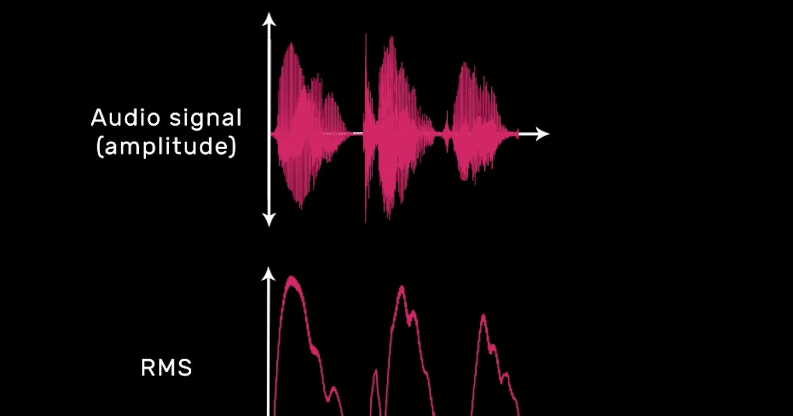
If volume is relevant to you, you should start with RMS. The RMS value of a set of values (or a continuous-time waveform) is the square root of the arithmetic mean of the squares of the values, or the square of the function that defines the continuous waveform. The diagram below shows the plot of an audio signal on top and the plot of the RMS for the audio signal on the bottom.

Source

You can see pretty clearly from the diagram above that the RMS gives us a higher value when the audio is higher in amplitude. As a very loose principle, a higher RMS means that we will perceive a sound as louder. However, our perception of loudness depends on all sort of complicated factors, so don’t take this as a hard and fast rule. But this can be good for things like detecting when a sound has started or estimating whether an instrument is playing quietly or loudly.

Waveforms made by summing known simple waveforms have an RMS that is the root of the sum of squares of the component RMS values if the component waveforms are orthogonal (that is, if the average of the product of one simple waveform with another is zero for all pairs other than a waveform times itself)

We’ve come to the end of day 032. I hope you found this informative. Thank you for taking time out of your schedule and allowing me to be your guide on this journey.

Reference

*https://www.kadenze.com/courses/machine-learning-for-musicians-and-artists-v/sessions/sensors-and-features-generating-useful-inputs-for-machine-learning*

*https://en.wikipedia.org/wiki/Root_mean_square*